Homework_08
clbenning
2025-03-24
Question 1: Working with fake data —-
library(ggplot2)
library(MASS)
## Warning: package 'MASS' was built under R version 4.4.2##
## Attaching package: 'MASS'## The following object is masked from 'package:dplyr':
##
## selectRead in a data vector
{r} # z <- rnorm(n=3000,mean=0.2) # z <- data.frame(1:3000,z) # names(z) <- list("ID","myVar") # z <- z[z$myVar>0,] # str(z) # summary(z$myVar) #
#### Plot a histogram of fake data
{r} # p1 <- ggplot(data=z, aes(x=myVar, y=..density..)) + # geom_histogram(color="black",fill="darkgoldenrod2",size=0.2) # print(p1) # ```` # # #### Add empiracal density curve #{r}
p1 <- p1 + geom_density(linetype=“dotted”,size=0.75)
print(p1)
# # #### Get the maximum liklihood parameters for normal distribution # #{r}
normPars <- fitdistr(z\(myVar,"normal") # print(normPars) # str(normPars) # normPars\)estimate[“mean”]
# # #### Plot the normal probability density on the histogram # #{r}
meanML <- normPars\(estimate["mean"] # sdML <- normPars\)estimate[“sd”]
xval <- seq(0,max(z\(myVar),len=length(z\)myVar))
stat <- stat_function(aes(x = xval, y = ..y..), fun = dnorm, colour=“red”, n = length(z\(myVar), args = list(mean = meanML, sd = sdML)) # p1 + stat # ``` # # #### Add the exponential, uniform, gamma, and beta probability density curves # # ```{r} # expoPars <- fitdistr(z\)myVar,“exponential”)
rateML <- expoPars\(estimate["rate"] # # stat2 <- stat_function(aes(x = xval, y = ..y..), fun = dexp, colour="blue", n = length(z\)myVar), args = list(rate=rateML))
p1 + stat + stat2
# #{r}
stat3 <- stat_function(aes(x = xval, y = ..y..), fun = dunif, colour=“darkgreen”, n = length(z\(myVar), args = list(min=min(z\)myVar), max=max(z\(myVar))) # p1 + stat + stat2 + stat3 # ``` # # ```{r} # gammaPars <- fitdistr(z\)myVar,“gamma”)
shapeML <- gammaPars\(estimate["shape"] # rateML <- gammaPars\)estimate[“rate”]
stat4 <- stat_function(aes(x = xval, y = ..y..), fun = dgamma, colour=“brown”, n = length(z\(myVar), args = list(shape=shapeML, rate=rateML)) # p1 + stat + stat2 + stat3 + stat4 # ``` # # ```{r} # pSpecial <- ggplot(data=z, aes(x=myVar/(max(myVar + 0.1)), y=..density..)) + # geom_histogram(color="grey60",fill="cornsilk",size=0.2) + # xlim(c(0,1)) + # geom_density(size=0.75,linetype="dotted") # # betaPars <- fitdistr(x=z\)myVar/max(z\(myVar + 0.1),start=list(shape1=1,shape2=2),"beta") # shape1ML <- betaPars\)estimate[“shape1”]
shape2ML <- betaPars\(estimate["shape2"] # # statSpecial <- stat_function(aes(x = xval, y = ..y..), fun = dbeta, colour="orchid", n = length(z\)myVar), args = list(shape1=shape1ML,shape2=shape2ML))
pSpecial + statSpecial
```
Question 2: Rye Data —-
This data is a compilation of performance metrics, agronomic practices, and soil properties across the eastern half of the United States. The dataset includes a total of 5,695 cereal rye biomass observations across 208 site-years between 2001–2022 and encompasses a wide range of agronomic, soil, and climate conditions.
Read in data set
library(readr)
ryedat <- read_csv("rye_data.csv")
## Rows: 5695 Columns: 27
## ── Column specification ──────────────────────────────────
## Delimiter: ","
## chr (12): site_id, year, rye_planting_date, rye_sampling_date, cultivar, rep...
## dbl (15): study_id, N_rate_fall_kg_N_ha, N_rate_spring_kg_N_ha, shoot_biomas...
##
## ℹ Use `spec()` to retrieve the full column specification for this data.
## ℹ Specify the column types or set `show_col_types = FALSE` to quiet this message.View(ryedat)
ryedat$study_id <- as.factor(ryedat$study_id)
ryedat$site_id <- as.factor(ryedat$site_id)Plot histogram of rye data
plot <- ggplot(data = ryedat, aes(x =  shoot_biomass_mean_kg_ha, y = ..density..)) +
  geom_histogram(color="black",fill="aquamarine3",size=0.2) +
  theme_classic()
## Warning: Using `size` aesthetic for lines was deprecated in
## ggplot2 3.4.0.
## ℹ Please use `linewidth` instead.
## This warning is displayed once every 8 hours.
## Call `lifecycle::last_lifecycle_warnings()` to see where
## this warning was generated.plot## Warning: The dot-dot notation (`..density..`) was deprecated in
## ggplot2 3.4.0.
## ℹ Please use `after_stat(density)` instead.
## This warning is displayed once every 8 hours.
## Call `lifecycle::last_lifecycle_warnings()` to see where
## this warning was generated.## `stat_bin()` using `bins = 30`. Pick better value with
## `binwidth`.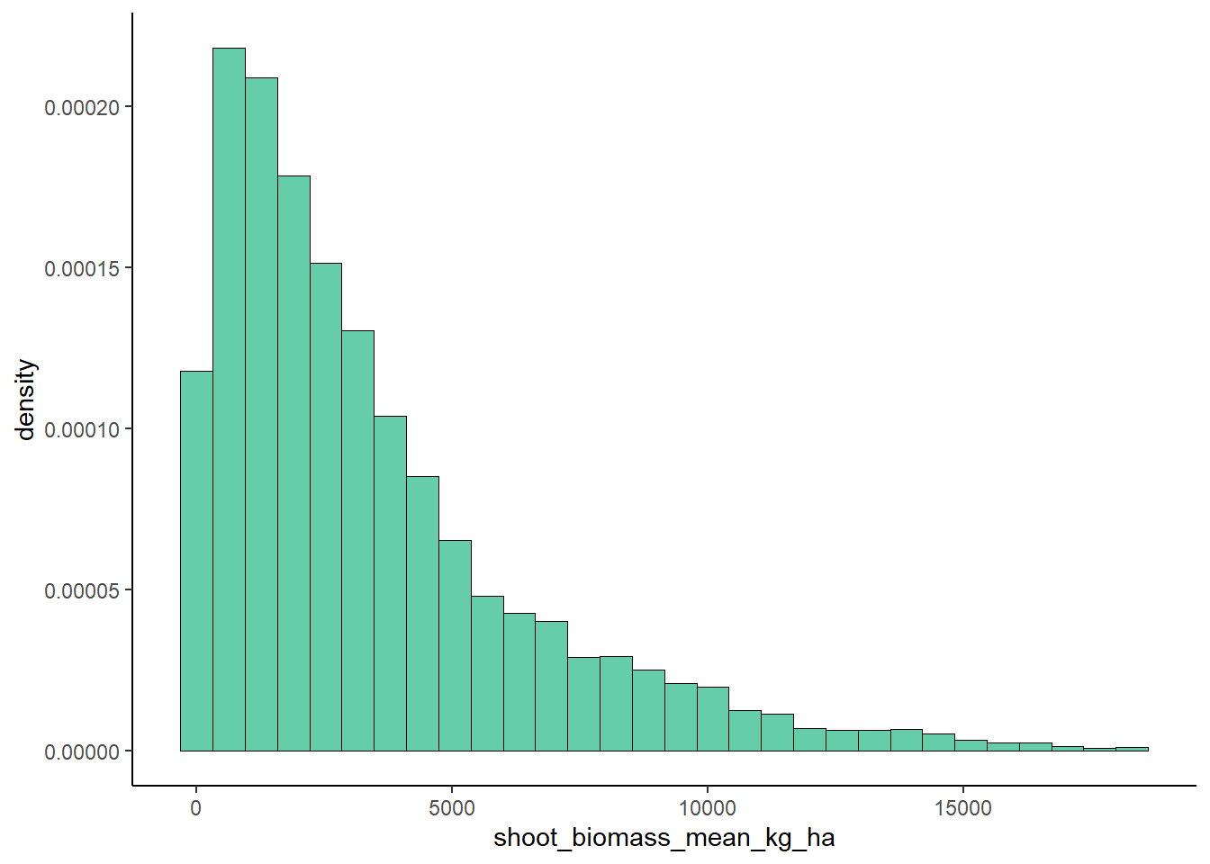
Emipirical Density Curce
plot <- plot + geom_density(linetype="dotted",size = 2)
plot
## `stat_bin()` using `bins = 30`. Pick better value with
## `binwidth`.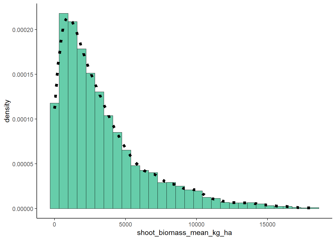
Maximum Liklihood Parameters for Normal
normPars <- fitdistr(ryedat$shoot_biomass_mean_kg_ha, "normal")
print(normPars)
## mean sd
## 3428.26191 3163.35061
## ( 41.91799) ( 29.64050)str(normPars)## List of 5
## $ estimate: Named num [1:2] 3428 3163
## ..- attr(*, "names")= chr [1:2] "mean" "sd"
## $ sd : Named num [1:2] 41.9 29.6
## ..- attr(*, "names")= chr [1:2] "mean" "sd"
## $ vcov : num [1:2, 1:2] 1757 0 0 879
## ..- attr(*, "dimnames")=List of 2
## .. ..$ : chr [1:2] "mean" "sd"
## .. ..$ : chr [1:2] "mean" "sd"
## $ n : int 5695
## $ loglik : num -53979
## - attr(*, "class")= chr "fitdistr"normPars$estimate["mean"]## mean
## 3428.262#Normal Distribution
meanML <- normPars$estimate["mean"]
sdML <- normPars$estimate["sd"]

xval <- seq(0,max(ryedat$shoot_biomass_mean_kg_ha),len=length(ryedat$shoot_biomass_mean_kg_ha))

stat <- stat_function(aes(x = xval, y = ..y..), fun = dnorm, colour="red", n = length(ryedat$shoot_biomass_mean_kg_ha), args = list(mean = meanML, sd = sdML))

plot + stat
## `stat_bin()` using `bins = 30`. Pick better value with
## `binwidth`.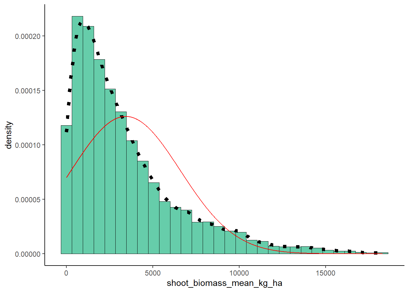
Exponential Probability Density
expoPars <- fitdistr(ryedat$shoot_biomass_mean_kg_ha,"exponential")
rateML <- expoPars$estimate["rate"]

stat2 <- stat_function(aes(x = xval, y = ..y..), fun = dexp, colour="blue", n = length(ryedat$shoot_biomass_mean_kg_ha), args = list(rate=rateML))

plot + stat + stat2
## `stat_bin()` using `bins = 30`. Pick better value with
## `binwidth`.
Uniform Probability Density
stat3 <- stat_function(aes(x = xval, y = ..y..), fun = dunif, colour="darkgreen", n = length(ryedat$shoot_biomass_mean_kg_ha), args = list(min=min(ryedat$shoot_biomass_mean_kg_ha), max=max(ryedat$shoot_biomass_mean_kg_ha)))

plot + stat + stat2 + stat3
## `stat_bin()` using `bins = 30`. Pick better value with
## `binwidth`.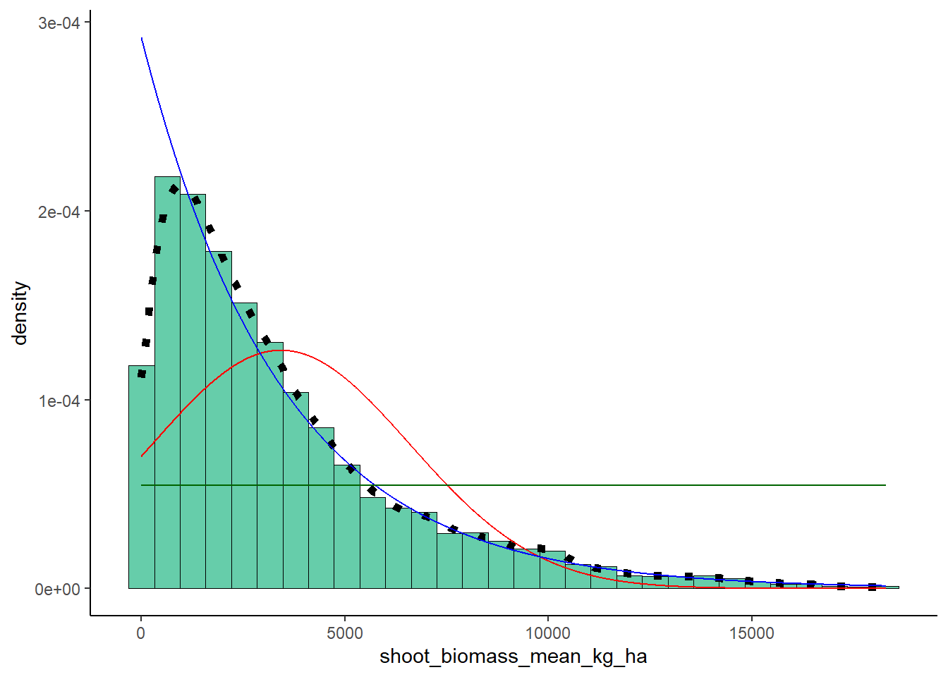
Gamma Probability Density
# gammaPars <- fitdistr(ryedat$shoot_biomass_mean_kg_ha,"gamma")
# shapeML <- gammaPars$estimate["shape"]
# rateML <- gammaPars$estimate["rate"]

# stat4 <- stat_function(aes(x = xval, y = ..y..), fun = dgamma, colour="brown", n = length(ryedat$shoot_biomass_mean_kg_ha), args = # list(shape=shapeML, rate=rateML))

# plot + stat + stat2 + stat3 + stat4